Google Sheets =COUNTIF Function

The =COUNTIF function is used in Google Sheets to detect duplicate data.

=COUNTIF Function to Find Multiple Criteria

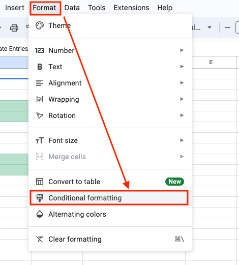
After opening the Conditional Formatting area, click on the “Add another rule” button.

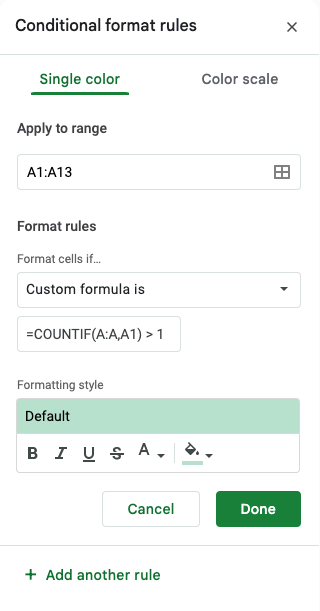
When specifying the cell range, it is marked in a matrix format. In the example below, to select only rows 1 to 13 in column A, paste the following code:

A1:A13

In the format rule area, select the “Custom formula is” option from the list of choices, and paste the following code:

=COUNTIF(A:A,A1) > 1

Finally, in the “Formatting style” area, choose what action to take when duplicate values are found (background color, bold text, underlined text, strikethrough text, etc.), and save it by clicking the save button. In this example, duplicate values will be highlighted in green.

How Does =COUNTIF Function Work?

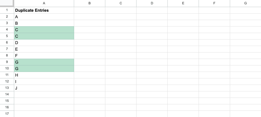
The function determines duplicate criteria as shown below.

You can review a sample sheet that uses the =COUNTIF function by clicking the button below.

=COUNTIF